 This page is under construction
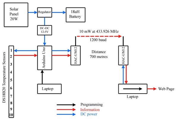 Block Diagram
This diagram shows the basic components required for collecting temperature readings from seawater and transmitting the data to a base station where it can be collated into a database for analysis. To the left is a schematic of 10 temperature sensors, spaced 1 metre apart and immersed in seawater to a depth of 10 metres. This is connected to an Ardiuno Uno microprocessor which has been programmed to collect the readings and pass them on to a radio transmitter. The Arduino board requires a 5V supply which is provided by a DC-DC converter. This is supplied by a sealed lead acid 12V battery and solar panel with regulator. The Arduino Uno board is programmed via a usb cable connected to a laptop, and of course is disconnected when the program is uploaded into the microprocessor. The Arduino Uno board passes the temperature data to a small radio transmitter which is received by a receiver about 700 metres away. This passes the data into a laptop via a serial/usb dongle. Software reads the incoming data and massages it in various ways and dumps it into a database. Some preliminary analysis is carried out and results sent to a web page.
The 'wet end' of the system at sea is automated to read the 10 temperature sensors 10 times in quick succession, send this data, and then go to sleep for 20 minutes to save power so that the solar panel can keep up with current drain from the backup battery. The battery voltage and number of hours of continuous operation are transmitted at the end of each radio transmission. Fluctuations in battery power are monitored with software at the 'dry end', the receiving station on land. This acts as an early warning that the solar panel may not be keeping up with power consumption so that action can be taken to avert interuptions in data flow.
During any one 24 hour period some 7,200 temperature readings are collected from 10 depths. The total data flow is quite modest: each transmission is 13.6 kb, or 0.98 mb per day. The two radios are factory programmed at 1200 baud to facilitate the most reliable passage of data to the receiver. Even so, occasional transmission errors occur. In such cases, examination of the characters received suggests the receiver has been swamped by RF from some other source. Automatic detection of such problems is relatively simple and is further discussed below.
The device will report temperatures in the range of -55 to 125°C, and is reputed to be accurate within the range ± 0.5°C, though exactly how this calibration on an absolute scale has been achieved is not clear. I have twice requested technical information from Maxim on this point and was simply re-quoted the statement of accuracy in the manual without further explanation. It would be an interesting experiment for first year university Physics students to test this claim. Thermal calibration usually involves using some fixed points like melting ice and boiling water, but controlling all the environmental variables to within ± 0.5°C and then measuring it is not an easy task. What would one use - perhaps a DS18B20?
A more important issue is the possibility of drift of various kinds, or reports from the device which vary during the length of time taken for interrogation, charge up of capacitor, heating of wire carrying current, etc. This is not a trivial matter when you consider that seawater temperatures at 10 metres depth are not likely to change quickly, depending on the exact character of tidal streams at a specific locality. Deciding whether a reported change of 0.5°C is real or not is not so simple.
There is a clear message here, 'dont believe everything you read in the newspaper'. A digital readout of 17.31°C is impressive, especially if it is only measured once. This is the reason why in the block diagram described above, each sensor is measured 10 times, and these 10 reports are sent to the 'dry end' for scrutiny. More of this later.
Each sensor has a unique 64-bit serial code stored in an onboard ROM. These must be identified so they can be used later during interrogation for temperature readings. Paul Stoffregen has written a software library which can be used by the Arduino Uno board for communicating with the DS18B20 sensor.
The ten sensors in the array being used here have these addresses:
Most of the companies manufacturing waterproof DS18B20 sensors make them with various custom lengths of coax attached, but one company, Shenzhen VIIV Technology Co. Ltd. in China, offered to make a one-off cable for me with 10 coax cables cut at lengths of 10m, 9m, 8m, etc and bundle all cables together and coat the outside of the stainless steel buckets with additional resin for enhanced corrosive resistance (see image to the right). The final overall length was 14m and cost US$190 including shipping. The contact person for this order was averil@szviivtech.com.
As mentioned above, this star configuration with multiple wires starting from one point, each leading to a sensor, raises a small problem. Depending on the total length of wire in the system, spectacular false readings of -127.00°C are sometimes generated, or simply 0.00°C. In cases like this the 4.7kΩ resister needs to be reduced to allow more current to flow to the wire which charges a capacitor inside the DS18B20 sensor. Paul Stoffregen suggested lowering the value to 1kΩ, and if this still failed to work to try 470Ω. I wanted to add an additional 10 metres of three wire cable on to the end of the bundled-up 10 coax cables for attachment to a distant box of electronics, so considerable experimenation was required to find the highest resistor that produced consistently reliable temperature reports. The final resistor was a 1% tolerance 480Ω resistor.
There is a total of 30 wires from the bundle of 10 coax cables requiring termination. Each of these was examined for continuity with somewhat surprising results. The DC resistance from the shield of each individual coax to each wire leading to the three terminals of each DS18B20 was found to be the following. NB: the ">" symbol is used when a resistance is off scale on the 2,000 MΩ range. These results suggest that there is a short between the GND wire and the shield in the case of the 3 metre cable. This shield also has a lower than expected resistance with both the VDD and DQ wires for this same cable. Whether this is a problem or not remains to be seen. Finally, coax cables for both the 8 and 9 metre lengths exhibit lower than expected resistance, although still very high.
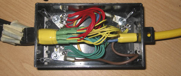
All the GND wires are soldered on to one single terminal in the termination box, and this was done with the VDD and DQ wires. A 10-metre-long three-wire heavy duty cable was then soldered to the same terminals and led away to the main box carrying the electronics. Although not shown in the image below this termination box is then filled with Sika Marine ISP-919 Silicone sealant. Although not immersed in seawater, this box is exposed to the elements for long periods and this treatment completely waterproofs the box and its contents.
David Pook of Westshore Marine Ltd kindly donated four litres of Altex Coating Industrial & Marine antifoul on the cable. The cable was coiled up and immersed in a large can of antifoul each morning and hung up to dry. This treatment was repeated over four successive days to ensure a thick coating on the cable. After the final coat it was left hanging for five days to ensure full hardening.
A useful guide to what one might expect from various sized solar panels in London and Edinburgh can be found here. These are average values with the solar panel mounted at optimum angle to the sun. The average sunshine in London is about 1,500 hours per annum, and for Edinburgh about 1,350 hours per annum. New Zealand values compare favourably to these. There are no estimates for Ngakuta Bay, but values for nearby locations are: Auckland and Wellington are both about 2,050 hours per annum, Nelson 2,400 hours per annum and Blenheim 2,500 hours per annum. A conservative estimate for Ngakuta Bay would be about the same as Wellington.
Previous reports of power consumption of the different components in similar recording systems vary widely. There are some reports of about 25 mA for the Arduino Uno board, but Windows 7 reports the USB root hub properties requiring 100 mA. The DS18B20 sensors are rated at requiring a maximum of 1.5 mA each when operating and 1 mA on standby. The radio transmitter being used is rated at 32 mA when receiving, 42 mA when transmitting, and 5 μA when in sleep mode.
Total power consumption was measured when using a battery delivering 12.2 V, and found to be 64.8 mA during the transmitting part of the cycle, 41.4 mA during the standby period, and 28.0 mA during sleep mode. One cycle consists of the following elements which were timed with a stop watch:
So we can estimate that during the winter solstice at Ngakuta Bay, approximately 1.12 * 0.725 aH would fall on our horizontal 20 watt solar panel, which is about 0.812 aH per day. Our calculated power consumption per day was 0.696 aH per day, so there appears to be about a 17% margin of safety in the solar panel rating for mid-winter. This is not a large margin, but hopefully will be enough.
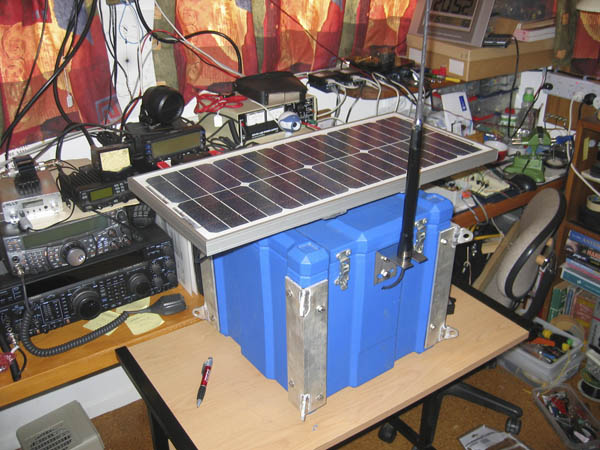
The main power source is a DiaMec DM1218 12V-18 aH sealed battery, and there is a MP3128 PV Solar Charge Controller between the battery and the solar panel. This controller is rated at 26 volt and 6A maximum rating. This battery and controller and all electronics are inside a special waterproof box with the solar panel mounted on the top (image above right). All external bolts and feedthroughs are covered with silicone sealant to ensure waterproofing. There are two rings on each corner of this box for tying it in a secure location on board the vessel at sea. All engineering is aluminium alloy with marine grade #316 stainless steel bolts and nylox nuts. The engineering costs were $367
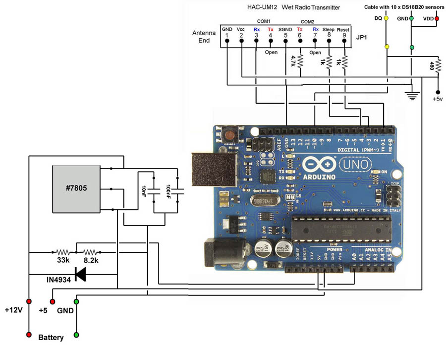
The two resitors shown near this power supply act as a voltage divider fed into Pin A0 on the Arduino Uno board. This provides digital data as a proxy of the condition of the 12V battery. More of this later. The input feed from the cable with the DS18B20 sensors shows the 480Ω resistor, discussed earlier. The value of this resistor was decreased from the standard 4.7kΩ normally used for the one-wire configuration also discussed earlier, and illustrated to the right.
The VDD wire is latched to earth as power to the sensors is being provided in parasitic mode. We experimented with providing power to the sensors on the VDD wire, but found this to be less reliable than parasitic mode with such long wires in the star configuration. The reason for this is not clear.
The digital data from the DS18B20 sensors comes in on Pin 10, and is sent out to the serial port on the Rx Pin 3 of a DB9 connector, while the Tx Pin 4 is left open. Instructions for sleep and reset are sent out from Pins 3 and 4 on the Arduino Uno board to Pins 8 and 9 on the serial connector. Note that the second set of Rx and Tx pins on the serial connector is unused, Tx Pin 6 is held high through a 4.7k resistor, and Rx Pin 7 is left open.
Given the hostile marine environment that this supposedly waterproof box containing electronics is to be kept in for long periods, it was thought desirable to include a humidity sensor, which could be monitored along with the output of temperature data. If moisture entered the container for any reason, this would be an early warning of such a problem and could be attended to before the problem became serious. A suitable device would be the AHT15 digital humidity sensor, readily available here. There is an Arduino library for this device. There are plenty of spare pins on the Arduino Uno board for input from such a device. This has yet to be implemented.
Analysis of DS18B20 Sensor Performance and Normalisation
After thinking about this or a while it was realised this was set by the resolution of the sensors, which, as noted above was set to 12 bits. According to the the manual the sensors report values
from -55 to 125°C, which is a range of 180°C. The 12 bit resolution would therefore be 180/4096, which is 0.044°C, which is near enough to 0.06°C
to be confident that this is the reason for this rather odd anomaly. It can be noted that 0.06*4096 would give a range of 246°C rather than 180°C as specified.
It will be recalled that the specifications for the DS18B20 temperature sensors state that they accurate to within ± 0.5°C of the correct temperature within the range of -55 to 125°C. Since this project is designed to detect temperature changes in water at different depths, it is important to know if, when any two sensors produce values that are ± 0.5°C apart, the difference is due to an actual temperature change or random variations within the device's level of tolerance. In other words, the absolute accuracy of these devices is not as important as their relative accuracy.
The Company that makes these devices has published no useful information on their relative accuracy, so it was decided to investigate this. It would be sensible to assume that there may be variations in relative performance between any one batch and another during manufacturing, so that one batch might consisently give values slightly above or below another batch, but hopefully still be within thre specified level of tolerance of ± 0.5°C. Two devices on the cable at different depths in the water might therefore appear to show slightly warmer or colder water where no such difference really exists.
The cable with the ten sensors was placed in a large plastic vat and filled with approximately 150 litres of fresh water to a depth of 30cm, and temperature readings were taken as described above (ten readings of each sensor every 20 minutes) for several days followed by analysis. Tne vat was placed on a concrete ground floor at the southern rear of the building away as far from the influence of daily sunshine as possible. It was hoped this would keep diurnal changes to a minimum.
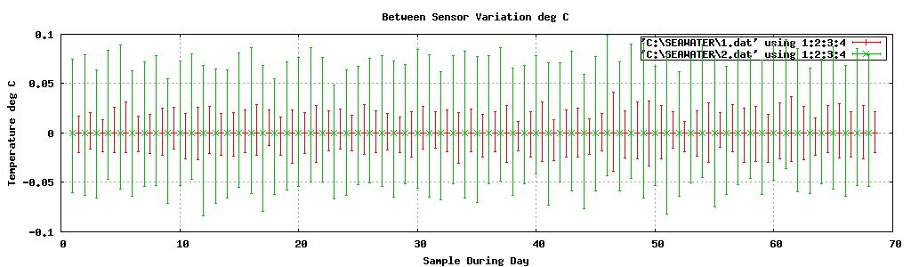
Consistent differences were found from one sensor and another. The experiment was repeated after raising the cable from the bottom of the vat to about half depth to avoid any bottom effects due to the underlying concrete floor. Much the same results were obtained, but it was noticed that the relative order of sensors recording above and below each other had changed from the first experiment. This suggested that the sensors were sensitive to a thermal gradient from bottom to top in the vat of water. This was confirmed by changing the relative heights of different parts of the cable and repeating the experiment several times. This is extremely good news, suggesting that very small differences in seawater temperature might be able to be detected if the different sensors could be normalised to read the same value in the same water temperature.
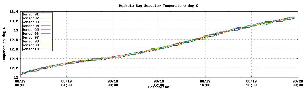
To facilitate thorough mixing of the water to get rid of any vertical gradient in temperature a submersible circulation pump was installed in the centre of the vat. This was model HQB-2000, rated at a throughput of 1400 litres per hour. This certainly cut down on variations between sensors, although diurnal changes were still significant. Moving the sensors around in the bath made no difference to the relative order of sensor readings, suggesting that thermal grandients were now minimal.
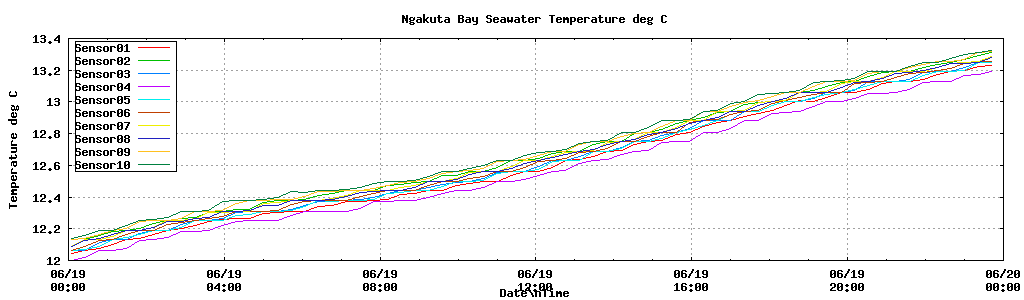
The graph below shows a typical record of freshwater temperature during a 24 hour cycle, showing a rise of 1.4°C throughout that period. Note that each sensor occupies a consistent relative position above or below each other sensor. This might be referred to as the batch effect relating to subtle differences during manufacture. These tiny changes could of course be partly due to the different incremental lengths of wire on the cable for each depth (see below). Also note that the total width of the band of temperatures recorded by the 10 sensors is approximately 0.1°C. Please note this does not challenge the device specification of ± 0.5°C. This smaller band shows that all sensors are reporting values within 0.1°C, even though on an absolute scale all values could be above or below the reported value, but within a band of ± 0.5°C.
 The Temperature Sensor
The heart of the system is a digital temperature sensor made by Maxim Integrated Products. The device is labelled DS18B20 because it was originally made by Dallas Semicondutors. Maxim acquired the Company in 2001 and continued the device name.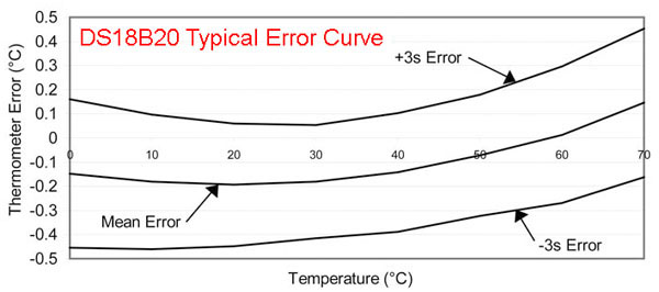
0x28, 0xD3, 0x0F, 0xE5, 0x03, 0x00, 0x00, 0xC0
0x28, 0x14, 0x07, 0xE5, 0x03, 0x00, 0x00, 0xE4
0x28, 0xCE, 0xF8, 0xE4, 0x03, 0x00, 0x00, 0xA9
0x28, 0x24, 0x10, 0xE5, 0x03, 0x00, 0x00, 0x24
0x28, 0x24, 0x03, 0xE5, 0x03, 0x00, 0x00, 0x16
0x28, 0x30, 0x10, 0xE5, 0x03, 0x00, 0x00, 0xA3
0x28, 0x78, 0xFC, 0xE4, 0x03, 0x00, 0x00, 0x03
0x28, 0xA8, 0x0D, 0xE5, 0x03, 0x00, 0x00, 0x23
0x28, 0x99, 0xDA, 0xE4, 0x03, 0x00, 0x00, 0x79
0x28, 0xA2, 0xE8, 0xE4, 0x03, 0x00, 0x00, 0x6B
Two software libraries are required when writing code for the Arduino Uno board to communicate with the DS18B20 sensors: OneWire and Dallas Temperature. Jim Studt created the original OneWire library in 2007, and this is now maintained by Paul Stoffregen. The latest version 2.1 can be downloaded from here. The second library, Miles Burton's Dallas Temperature Control library can be downloaded from here. These libraries are open source software.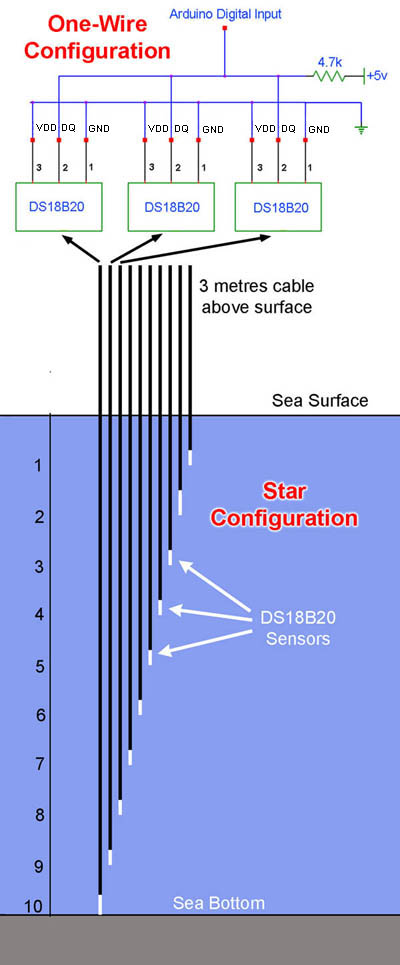 There are three terminals on the DS18B20 sensor: GND, DQ, and VDD. The device can be powered directly by the DQ Data Line, requiring 3.0V to 5.5V. If this is done, the VDD terminal can be strapped to GND, as shown in this diagram to the left. The thermometer resolution is user-selectable from 9 to 12 bits, and it converts temperature to a 12-bit digital word within 750 ms. When several sensors are being used, they may be mounted on a single rail as shown. A request from the Arduino Uno board to this rail for a temperature reading using one of the serial codes above returns the value from the appropriate individual sensor. This is referred to as the One-Wire Configuration. Strictly speaking two wires are required of course, the DQ and GND wires. This configuration is easy to assemble on two wires, but if waterproofing is required it is not at all simple. Coating two wires with multiple sensors attached with shrink-wrap might be splash proof, but it certainly would not be waterproof, especially if immersed in 10 metres of seawater with a surrounding fluid pressure of 1,000 mbar. This is the difference between a water resistant watch which is splash-proof, and a diving watch which is genuinely waterproof under pressure with ISO-6425 rating.
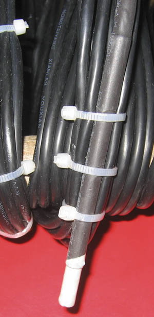 It would be possible to make a single waterproof cable with multiple sensors on it, but it would be quite complicated. A much simpler design is the so-called Star Configuration, also shown to the left. This involves running separate cables to each sensor and joining them on to the one wire rail at the far end from the longest cable. This is much easier to waterproof, although another problem arises, though relatively easier to solve than with the one-wire configuration. Fortunately, there are numerous manufacturing companies making waterproof versions of the DS18B20 sensor. The sensor is attached to a coax cable with three wires soldered on to the sensor terminals and the sensor and bare wires are then inserted into a stainless steel tube bucket and filled with thermally conducting resin, thus waterproofing the metal parts of the sensor and wires. The special resin assists with transferring thermal enegery from the surrounding environment through the stainless steel to the sensor itself. Unfortunately, marine #316 grade stainless steel is not used by these companies, but the less corrosion resistent #304 grade. In addition, as is well known, stainless steel is a very poor conductor of heat, so we can expect a small time-lag in the sensor respoding to temperature changes in the surrounding seawater. Stainless steel #304A grade has a thermal diffusivity (the measure of thermal inertia) of 4.2 mm2/s compared to copper of 110.8 mm2/s. What the additional time-lag is as a result of using the thermally conducting resin is not known.
Metres
VDD
DQ
GND
1
>
>
>
2
>
>
>
3
11MΩ
10MΩ
76Ω
4
>
>
>
5
>
>
>
6
>
>
>
7
>
>
>
8
c.300MΩ
c.300MΩ
c.300MΩ
9
c.300MΩ
c.300MΩ
c.300MΩ
10
>
>
>
 Antifoul Protection of the Cable
Because the monitoring cable was scheduled to be immersed in seawater for up to two years it was necessary to coat the cable with marine antifoul paint to deter organisms from growing on it. Moorning lines in Ngakuta Bay attract both green-lipped and blue mussels (Perna canaliculius and Mytilus galloprovincialis ) as well as numerous other smaller species. The Cable was attached to a 15 metre long 1cm diameter polyester double braid rope which has minimal stretch using nylon self-locking fasteners. A zinc anode was attached to the end of the rope weighing 2.6 kg. This is designed to hold the cable vertical in the water.
 Solar and Battery Power Supply
Running electronic equipment 24 hours a day and 365 days of the year from a battery with re-charging by solar panel requires careful attention to current use and a conservative estimate of delivery from sunshine.
Location
Solar Panel output
Summer aH per day
Winter aH per day
London
10 watts
3.41
0.41
London
30 watts
10.4
1.14
London
60 watts
20.9
2.29
Edinburgh
10 watts
3.21
0.22
Edinburgh
30 watts
9.55
0.67
Edinburgh
60 watts
19.1
1.32
Step 1: collect and transmit temperatures from each of the 10 sensors, taking 1.99 seconds.
A complete transmitting and standby cyle therefore takes (1.99+4.69)*10 = 1 minute 6.8 seconds, with 20 minutes sleep, totalling 21 minutes 6.8 seconds. Each transmitting cycle is time-stamped, and the average gap between them is 21 minutes 10 seconds, which accords well with the stop watch values. During any one 24 hour period there are approximately 68 full cycles. The total power consumption during a 24 hour period can thus be calculated as follows:
Step 2: standby, taking 4.69 seconds.
repeat steps 1 and 2 ten times, then
Step 3: sleep for 20 minutes.
Step 1: 64.8 mA for 1.99 seconds = 0.0358 maH.
The total daily power consumption is therefore apportioned as follows:
Step 2: 41.4 mA for 4.69 seconds = 0.0538 maH
repeat steps 1 plus 2 ten times = 0.8962 maH, followed by
Step 3: 28.0 mA for 20 minutes = 9.3333 maH
which is a total of 10.2296 maH per full cycle
The 68 cycles per 24 hour period would therefore consume 695.6115 maH
Transmitting = 24.3576 maH, 3.5%
These are very interesting results. Clearly, the power consumption actually doing anything is trivial compared to the amount of power being used sitting around waiting to do something. What might we expect from the solar panel becomes the next question. We can expect about the same sunshine hours at Ngakuta Bay as the lower New Zealand values of Wellington and Auckland at about 2,050 hours per annum, or about 1.37 times the values for London at 1,500 hours per annum. The average yield in London of a 20 watt solar panel during winter would be about twice the value for 10 watts (0.41*2), say 0.82 aH per day, which should correspond to approximately 1.37 times that value for Ngakuta Bay, or 1.12 aH per day. However, it will be remembered that the London values were with the solar panel mounted at optimum angle to the sun. This will not be possible with the array being used here. The solar panel along with the electronics and cable in the sea will be mounted on a private vessel moored in Ngakuta Bay. The vessel will move about on the mooring line during the day 360°, and the best possible angle for the solar panel will be flat horizontal to catch the greatest sunshine. The angle of the sun at various times of the year at Wellington, which is very close to the Latitude at Ngakuta Bay, is well documented. The best time of the year is the summer soltice on December 22 at 72.2° elevation, followed by the two equinoxes of March 21 and September 23 at 48.7° elevation, and the winter solstice of June 22 at 25.2° elevation. The solar energy falling on a horizontal panel when the sun angle is 25.2° elevation would be approximately 72.5% of that which would fall on a panel at the optimum angle to the sun.
Standing by = 36.5872 maH, 5.26%
Sleeping = 634.6667 maH, 91.24%
Total = 695.6115 maH, 100.00%
 The Arduino-Uno Board
After considerable experimentation, this schematic on the right shows the final wiring of the Arduino Uno board to power supply, radio transmitter, and the cable with DS18B20 sensors. The Arduino Uno board has an on-board 12V to 5V converter but it was thought there might be some power savings by having an external switchmode DC-DC power supply based on the #7805 converter.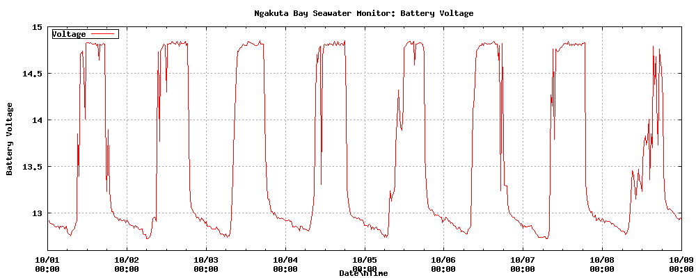 Keeping an Eye on Battery Power
It is hoped to monitor the 10 temperature sensors continuously for a minimum of two years, and clearly one of the most important factors is continuity of power supply from the battery. Although every effort was made to build in safety margins, a long period of low-level sunshine could prevent the solar panel from charging the battery to an acceptable level. For this reason, battery voltage is transmitted along with temperature data and continuously monitored. The information is automatically uploaded to this web page every day during each monthly cycle. An alarm system has been implemented in the software as an alert that attention is needed out on the water. The rising and setting of the sun are evident in the graph on the left.
 The Radio Transmitter and Receiver
There are many low power transmitter receiver modems available on the market. Those eventually chosen are manufactured by Shenzhen HAC Telecom Technology Co. Ltd in China. The contact person was shelly@rf-module-china.com and the cost was US$118 including shipping for four radios (two factory-set at 1200 baud and two at 9600 baud). The manual suggests that for the 9600 baud model reliable communication is greater than 300m when the antenna height is at least 2m, and greater than 500m if the antenna height is more than 5m. However, another document released by the Company states this:
Within the visible range, when the height of antenna is higher than 2m and The Bit Error
Rate (BER) is 10-3, the reliable transmission distances respectively is 1000m@1200bps.
When the baud rate is 4800bps, it is more than 700m. When the baud rate is 9600bps, it is
more than 500m.
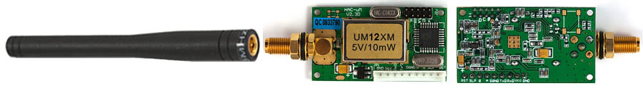
These radios with different baud rate are identical but factory set to the specified baud rate and labelled thus. It is expected that the electronics will be stationed on one of three different vessels in Ngakuta Bay, and moved from one to another when one is required for other use. The receiving station is 550 metres from the closest vessel and 650 metres from the most distant. It was decided that it would be wise to install the 1200 baud radios for this task, HAC-UM12XM. These were tested in line of sight from the receiving station to a roadway on a hill just over 800 metres distant and performed well, transmitting and receiving temperature data from ten DS18B20 sensors on a breadboard.
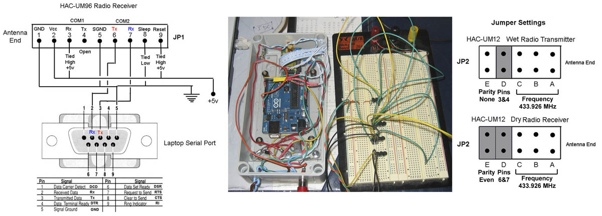
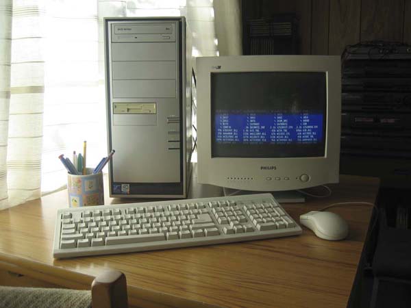
The image above shows the wiring for the receiver and jumper settings for the two radios. Instructions in the manual are not well rendered in English, but with perseverance can be understood. These radios are inexpensive and definitely work well at considerable distance, in spite of their low power of only 10 mW. When all jumpers are off for A,B,C, the frequency is set at 433.926 MHz, and the manual states the bandwidth as 12 kHz for the 1200 baud version. A reception test with a TS-2000X showed no signal at 433.920 MHz and a steep rise towards 433.926 MHz.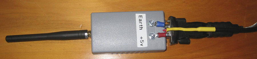 The receiving radio was mounted in a small box with a DB9 serial connector at one end. This is connected to a serial/usb dongle which works satisfactorily under Windows 7. During testing, the data were received using Teraterm with COM2 chosen and 1200,8,E,1 port settings. The voltage requirement is +5V and is rated at only 32 mA when receiving. The computer USB port is rated at 100 mA, so it was decided to use a second USB port to supply power from the computer. The end connector of a spare USB cable was cut off, and the two data wires (white and green) were cut short and each terminated with shrinkwrap. Voltage is carried with the red (+5v) and black (GND) wires. This arrangement works fine.
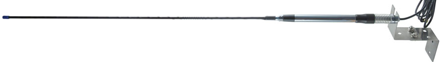 It was decided that in the interests of reliability, the two rubber duck antennas should be replaced by something with better characteristics. After considerable searching it was decided to splash out and buy two low angle omni-directional antennas made by an Australian Company called Elsemar (Electronic Service and Manufacture). It is expected that these antennas will have other uses after the seawater temperature monitoring project has been completed in several years' time. The antennas are 1 metre long with 3.6 metres of coax cable and terminated with an RP-SMA fitting, which plugs directly into the HAC-UM12 radios. The metal fittings are #304 grade stainless steel which is not the most suitable for marine applications, so these were covered with additional shrink-wrap. The frequency range is 428 to 437 MHz, with a tuned bandwidth of 9 MHz and a gain of 6.0 dBi. The SWR curve is less than 1.5:1 in the range of 430 to 435 MHz. The cost for two antenna: ANT433m and ANT433mspr (with base spring) was Au$166.65 including shipping. In their final position, the base of the transmitting antenna will be 2 metres above water level, and the receiving antenna will be 10 metres above ground level.
The temperature data is reported with a precision of two decimal places from the Arduino board and transmitted to the receiving station. It is was noticed that the decimal fraction of °C was not unformly distributed from 00 to 99, and this initially seemed puzzling. An analysis of one day's data showed incremental values clumped 0.06°C apart (eg: 0.13°C. 0.19°C, 0.25°C etc.) with no occurrences in between.
 Computer Software